PNAS – Tutorial Genomics, Ecology, Evolution, etc

Reconstructing human population history : ancestry and admixture

Thu, 31 Mar 2016 16:43:41 +0000

Understanding the evolutionary history of our own species, how migration and mixture of ancestral populations have shaped modern human populations is a key question in evolutionary biology. Here we present three articles related to this topic, the first two dealing with India and the third one focusing on a single Ethiopian group :

1) Moorjani et al 2013 Genetic Evidence for Recent Population Mixture in India AJHG 93,: 422–438

2) Basu et al 2016 Genomic reconstruction of the history of extant populations of India reveals five distinct ancestral components and a complex structure PNAS online before print

3) Van Dorp et al 2016 Evidence for a Common Origin of Blacksmiths and Cultivators in the Ethiopian Ari within the Last 4500 Years: Lessons for Clustering-Based Inference PLOS Genetics 11(8): e1005397

All of them use genome wide data from micro array. After a brief abstract of each paper, showing their similarities and differences, we discuss their methodological approaches.

Ancestral populations of India

The aim of the first two articles is to understand the history of the populations of the Indian subcontinent. The first one (Moorjani et al 2013) reports data from 73 groups living in India for more than 570 individuals sampled. The authors filtered out the data by removing all individuals with evidence of recent admixture or recent ancestry from out of India. The populations that were included in the analysis can be classified into two linguistic categories: the ones speaking Indo-European languages and the ones speaking Dravidian languages.

Figure 1 : map of sampled population (A) and PCA of 70 indians groups and some non-indians, highlighting the “Indian cline” (B)

Previous genetic evidence indicates that most of the groups of India descend from a mixture of two distinct ancestral populations: Ancestral North Indians (ANI) and Ancestral South Indians (ASI). Three different hypothesis exist for the date of mixture of these two populations:

1) arrival of ANI is due to migration prior to agriculture about 30,000-40,000 years ago

2) ANI arrived with the spread of agriculture who probably began around 8,000 and 9,000 years ago

3) ANI arrived very recently (3,000-4,000 years ago) when the Indo-European languages presumably began to be spoken in India.

To prove the admixed origin of Indian groups and estimate the proportion of each ancestry in each population they use a PCA and a statistic called F4 ratio that infers the mixture proportion measuring the correlation in allele frequencies between each pair of groups. They demonstrated that all populations are admixed and lie along an “Indian cline”, that is a gradient going from 17% of ANI ancestry to 71%. These results correlate well with geography and language, with the northern Indo-European populations having more ANI ancestry than the southern Dravidian ones. Then they use linkage disequilibrium (LD) to estimate the dates of admixture : LD blocs are longer if the admixture is younger. By fitting an exponential function to the decay of LD (that is expected from a sudden cessation of admixture) they could estimate that admixture occurred between 1,856 and 4,176 years ago, supporting the third hypothesis. These results correspond with demographic and cultural changes observed in India with the establishment of the caste system leading to strong endogamy that stopped the admixture rapidly. Moreover they found that Indo-Europeans groups have more recent admixture dates, which could be explained by multiple waves of mixture in these populations. Another finding of this paper is that aboriginal Andaman Islanders (Onge) belong to a sister group of ASI.

The second article (Basu et al 2016) has the same focus region and use the same basic dataset, except that the authors kept the all populations in the analyses, including the austro asiatic (AA) and tibeto burman (TB) speakers. They first ran ADMIXTURE on all populations and showed that islanders and mainland populations have distinct ancestral components (islanders share ancestry with oceanic peoples like Papuans). In a second time they ran the same analysis on mainland populations only (thus excluding population from the Andaman and Nicobar islands). The best model was composed of four ancestral components, the ANI, the ASI as well as the ancestral AA and TB and they found that several present day populations are almost pure representatives of these ancestral components (figure 2).

Fig. 2 : PCA of the 18 mainland Indian populations, the four clusters identified by the authors are surrounded (A). Admixture plot of mainland Indian populations with four ancestral components (K = 4, the most parsimonious) (B).

They further estimated the time and extent of admixture using the degree of fragmentation (due to recombination) of haplotypes blocs originating from a donor population into the recipient population. In each population, the distribution fitted again with an exponential curve. They showed that admixture abruptly came to an end about 1575 years ago in upper-caste populations, most likely due to the establishment of endogamy, while tribal populations seemed to have admixed until 1500-1000 years ago.

In short, although they share a common topic, these two papers propose divergent versions of the history of Indian population : while the first considers a priori that austro asiatic and tibeto burman speakers are not component of the ancestral populations of India and only focuses on the mixture between the ANI and ASI components, the second paper claims that the genetic structure of Indian population is the result of admixture events between four ancestral components. However the two views converge on the idea that admixture was a common phenomenon in India that ceased rapidly with the establishment of the caste systems that enforced endogamy.

Common origin of two subgroups of Ari people

The 3rd paper investigates the history of human populations at a smaller scale, focusing on a single ethnic group, the Ari people of Ethiopia. The Ari are composed of two socially and genetically distinct subgroups : the cultivators (Aric) and the blacksmiths (Arib). Anthropologists have proposed two alternatives hypothesis to explain the division of the Ari : under the remnant hypothesis (RN), the blacksmiths are the remnants of an indigenous group that was assimilated by the more recently arrived cultivators, whereas the marginalization (MA) hypothesis proposes that the two groups share a common ancestry but the blacksmith were recently marginalized due to their activity. While anthropologists traditionally favour the MA hypothesis, recent genetic studies have provided support for the RN hypothesis. In this article the authors use a new methodology on the same genetic dataset to bring evidence for the MA hypothesis. They show that when ADMIXTURE, fineSTRUCTURE or CHROMOPAINTER analysis are run on a complete dataset of 237 samples of 12 Ethiopian and neighbouring populations, the Arib are grouped into a single homogeneous cluster. But when the patterns of haplotype sharing are inferred by composing the Ari as a genetic mixture of all other groups, except themselves, the genetic differences between Arib and Aric disappear. In fact, their analyses reveal that the two Ari groups have the same mixture events with non Ari populations (figure 3).

Fig. 3 : Top : Inferred ancestry composition of recipient groups when forming each group as mixtures of (a) all sampled groups, (b) all sampled groups except the Ari. Bottom : TVD XY values comparing the painting profiles for all pairwise comparisons of groups X, Y under each analysis, with scale at far right. Ari groups (ARIb/ARIc) are highlighted with black outlines in each plot.

To explain this pattern they propose that the genetic differentiation of the blacksmith is due to a bottleneck effect. Their hypothesis is supported by the fact that identity-by-descent (IBD) is stronger in blacksmiths than cultivators which is consistent with reduced genetic diversity in the blacksmiths. Using the D-statistic, they also show that the Arib and Aric are more closely related to each other than they are to any other Ethiopian group. Therefore they conclude that the observed genetic differentiation between the Arib and Aric does not represent separate ancestry but is rather the result of strong genetic drift due to a bottleneck effect induced by the social marginalization of the blacksmiths.

Methodological discussion

What stands out from reading these three articles is that selection of a proper methodology is crucial within an hypothesis testing framework. While the two articles on Indian populations use the same initial dataset, the way they filter and analyse it results in very different conclusions. The inclusion or exclusion of some populations from an admixture analysis or outgroup selection for an f4 ratio estimation directly impact the output of these analysis and can lead the authors to tell very different stories. Before disclaiming or putting forward one hypothesis, it is important to be aware of the limitations of the method that is used to produce the results. For example the authors of the second paper on India’s ancestral populations, claim to demonstrate a more complex history than shown in the first paper but their result is solely based on a clustering analyse (implemented in various softwares such as STRUCTURE or ADMIXTURE).

The basic principle of those STRUCTURE/ADMIXTURE like programs is to take the K most different groups of the dataset, consider them as the pure ancestral groups and force the others to be a combination of those. This means that the results depend on the populations and the number of clusters K that are input in the program. There are different methods to determine which K provide the best fit to the data (cross-validation error, delta K …) but in numerous cases the inferred mixture proportions are wrong. Only in very simple cases, like the African American genetic history (well explained in Daniel Falush’s blog) that involves three clearly defined and very differentiated ancestral populations (West Africans, Europeans and Native Americans) we can be confident in the results of the clustering analyse.

Fig. 4 : Admixture plot of African American population (ASW) with his three ancestral populations, West Africans(YRI), Europeans (CEU) and Native Americans (MEX). Source : Daniel Falush’s blog

But in many cases the history is more complex and no current population actually corresponds to a pure ancestral population because of multiple waves of admixtures. In this case the most differentiated groups correspond only to the most extreme groups but it does not mean that these groups are pure or ancestral. This is well explained in Razib Khan’s blog using the simple example of Uygurs and Europeans : it is known that the Uygurs are a recently mixed group (between European and Asian) but if K is fixed to 2 with Uygurs and Europeans, STRUCTURE will form two different clusters at 100% levels, one with the Uygurs and one with Europeans. This is why, in the 2nd paper, the apparently pure AAA, ATB, ASI and ANI populations and all the clustering implications are probably meaningless. In fact, when using the f4 ratio (as in the first paper) all groups are found to be admixed to a certain extent (with the smallest rate of admixture being 17%).

This critic of clustering analysis is a key element of the study on the Ari people where the authors point out that results from such methods should not be taken for granted but interpreted with caution. Indeed this kind of method cannot discriminate between alternative scenarios of recent mixture of separate populations or shared ancestry followed by population divergence. Therefore support for one of these hypotheses should rely on additional tests. Instead of directly accepting the story suggested by a clustering analysis, a more reasonable work-flow would be to use other methods in order to address the specific implications of one hypothesis. This is exactly what is done in the third article where, as we previously explained, the authors constrain the analysis of mixture by forbidding self ancestry in the two groups of interest which remove the confounding effect of recent bottleneck. In such complex cases, associating PCA and STRUCTURE-like analyses with F-statistics and simulations allow to draw a more robust conclusion. Indeed statistics such as Fst or Dxy that estimate the genetic differentiation between two populations can be simulated under alternative scenarios, representing competing hypothesis (figure 5). These simulated statistics can be subsequently compared with the ones estimated from real data to favour one hypothesis over the other. Simulations can also give an idea of how difficult it is to discriminate between the different hypothesis, which avoid over interpretation of the results. In the second paper, where the authors put forward an new hypothesis, radically different from the classical hypothesis of anthropology and other genetic studies, additional tests like these seem necessary to strengthen their conclusions.

Fig. 5 : Differences in inferred ancestry under analyses A and B using F XY from real data on the top and from simulated data on the bottom (under MA and RN hypotesis). Here the MA hypothesis is obviously the closest to the reality.

Although it was not mentioned in any of the articles, the quality of the data and the way to obtain them, i.e. the kind of sequencing methodology, should also be a matter of precaution. Indeed, they all use micro arrays designed from European populations. These micro arrays consist of thousands of DNA spots containing a predefined sequence, known to be polymorphic in Europeans and only the complementary sequence can fix to this spot and be sequenced. So using these micro arrays to study the history of non european populations may be problematic as only SNPs that are variable for europeans will be targeted, probably leading to the exclusion of meaningful information for non European populations. Today, with New Generation Sequencing (NGS) there are many alternatives, such as RAD sequencing or Whole Genome Sequencing, that allow to sequence tens of thousands non-predefined SNPs.

Conclusion

To conclude, the take home messages from these three articles are :

– Social systems leading to endogamy can influence and modify rapidly and dramatically the genetic structure and patterns of humans populations.

– It is difficult to reconstruct the ancestry of human populations, especially when they involve a complex process with multiple waves of admixture.

– Clustering methods are designed to find a structure in a genetic dataset but they do not necessarily reflect real shared ancestry. Further test using other methods are required to robustly support one hypothesis.

]]>

The evolutionary history of polar bears

Tue, 18 Sep 2012 17:55:00 +0000

The study of the Ursus lineage, including brown bear (Ursus arctos), black bear (Ursus americanus) and polar bear (Ursus maritimus), provides the ability of addressing the subject of adaptation to extreme (salty and glacial) environments in mammals. Moreover, in last few decades, polar bears won public and media attention, being one of the most charismatic species endangered by global warming and Arctic ice melting. To trace history of innovations and determine response to environmental changes in populations of polar bears, two articles published in Science and Proceedings of the National Academy of Sciences in April and June 2012 provide new data and insights to resolve this question.

The absence of fossil of polar bears dating before the late Pleistocene (circa 126 000 years ago) and mitochondrial data, suggesting that polar bear were very closely related to a group of brown bear living in Admiralty, Baranof and Chichagof (ABC) islands in Alaska, previously led to believe that polar bears recently emerged from brown bears. The consequences of this hypotheses would be :

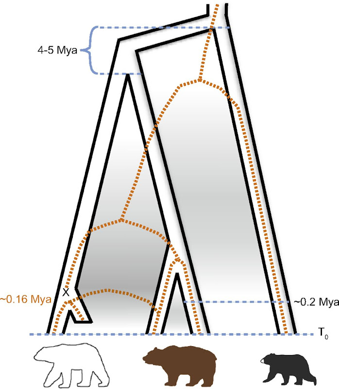
Polar bear underwent a very rapid and recent (less than 200 ky ago) adaptation to extreme environment (previously not seen in mammals)
Brown bear is a paraphyletic taxon, as polar bear is the sister specie of the ABC bears (see Fig. 1)


Fig. 1: Miller et al., Polar and brown bear genomes reveal ancient admixture and demographic footprints of past climate change, PNAS 2012

Phylogeny of bear lineage with mitochondrial DNA and Bayesian maximum clade credibility model

The blue box contains polar individuals coming from Svalbard and Alaska and an ancient sample 130ky to 110 ky old, the yellow box ABC individuals and the pink box other brown bear individuals. The outgroup is made of black bears individuals.

Nevertheless, both fossil data, as it can be incomplete, and mitochondrial data, as it sensitive to hybridization, are not sufficient to confirm this hypothesis. Thus the two publishing groups led in parallel projects aiming to collect nuclear data and test its agreement with mitochondrial data.

Hailer et al., in their work Nuclear Genomic Sequences Reveal that Polar Bears Are an Old and Distinct Bear Lineage published in Science, sequenced 9116 nucleotides from 14 independent introns in 45 individuals of black, brown and polar bears. Introns were sequenced to provide more variation between individuals: given the low amount of time since the divergence of the last common ancestor of bears (estimated between 559 to 1 429 ky ago in their study), choosing exons, whose evolution being more likely bounded by selection, would have yielded less information.

Using this data and various phylogenetic reconstructions (bayesian multilocus coalescent approach, bayesian inference for the concatenated data and neighbour-joining of the differentiation estimates between species) that all led to the same conclusion, they recovered the three species of bears as being monophyletic and observed in the species tree the polar bear clade being sister to the brown bear clade. They estimated the divergence time of the two species around 603 ky ago (338 to 934 ky being the 99% highest credibility range) and clearly revealed a discrepancy with the mitochondrial data.

The authors resolved this incongruence by stating that the most probable scenario was a divergence between polar and brown species 600 ky ago and an hybridization event between 111 to 166 ky ago between polar bears and ABC bears leading to the complete replacement of the former mtDNA by the latter. The opposite phenomenon (several and severe introgression events of polar bears mtDNA into brown bears leading to all extant mtDNA being of polar origin) is judged very unlikely by the authors given the extended range of distribution of the brown bear. The lack of finding of older fossil from polar bears was explained by their constantly changing living environment.

Despite the recent hybridization event, Hailer et al. found very few common nuclear haplotypes between polar and brown bears: out of the 35 polar and 79 brown haplotypes, only 6 of them were shared across both species. Nevertheless, we must bear in mind that given the relatively low amount of nuclear data analysed, those findings might not reflect the entire picture of polar and brown bears nuclear DNA ancestry.

In Polar and brown bear genomes reveal ancient admixture and demographics footprints of past climate change, published in PNAS by Miller et al., a genome-wide sequencing project was adopted to unravel the same problem. In this extensive study, the authors assembled a reference genome of a polar bear individual, deeply sequenced the genome of two ABC, one black and one non-ABC brown bear (GRZ). Finally, they produced low coverage data from 23 other polar bear individuals, one of them being an ancient specimen 110 to 130 ky old found in Svalbard.

Having aligned all reads from every samples to the polar bear genome reference, they identified 12 millions of what they called “SNPs” (even though they are dealing with three different species) and constructed the following phylogeny (Fig. 2).

Fig. 2: Miller et al., Polar and brown bear genomes reveal ancient admixture and demographic footprints of past climate change, PNAS 2012

Phylogeny based on the matrix of distances of the 12 millions SNP and using a neighbour-joining algorithm (probably given the amount of data and computational time needed with more sophisticated algorithms)

We observe that, as in the previous paper, the nuclear data is not in agreement with the mitochondrial data. A scenario where polar bears emerged as a sister species of the brown species and later experienced a massive and unique event of mtDNA introgression from ABC bears (as the polar bear individuals form only one group in Fig. 1) is again strongly favoured. Regarding the ancient polar bear specimen, both trees inform us that it dates after the mtDNA introgression event and that the modern individuals living in Svalbard are actually more closely related to the modern individuals in Alaska than to the ancient one.

Though up to this point both articles seem consistent, following findings radically differ with the previous study. Indeed, Miller et al., used a coalescence hidden Markov model for four of their deeply-covered genomes (one ABC, one polar bear, one brown bear, one black bear) to assess the history of the lineage. They estimated both the splits of polar bears with brown bears and the common ancestor of those two species with black bears to have occurred around 4 to 5 My ago, as shown in Fig. 3.


Fig. 3: Miller et al., Polar and brown bear genomes reveal ancient admixture and demographic footprints of past climate change, PNAS 2012

Reconstructed evolutionnary history of polar, brown and black bears

The black solid line represent the specie tree and the brown dashed lines the mtDNA tree

The X represents the introgression event, the shortened branch of the specie tree the disappearance of the ancient Svalbard lineage

It is however true that Hailer et al. reported on their article (that pre-dates the PNAS one) that other studies hint that the 600 ky-value is an underestimate of the splitting time of the two lineages under consideration, without it weakening their own conclusion.

Nevertheless, other discrepancies arise : Hailer et al. stated that no evidence of on going gene flow was found between polar bears and brown bears, whereas the coalescent model used by Miller et al. yielded that the time when this gene flow stopped was not significantly different from zero. Following the Science article, a comment arose relating two very recent cases of documented hybridization of polar/brown bears in the wild, among them a second generation hybrid. Interestingly, both crosses involved a polar bear female with a brown bear male: thus no cross leading to the introgression of brown bear mtDNA onto polar bear populations has yet been described.

Besides, where Hailer et al. found relatively few shared nuclear data between polar and brown bears, a PCA analysis of the SNPs identified in the ABC, non-ABC and polar bear genomes yielded that 5.5% of one of the ABC genome and 9.4% of the other one are related to the polar bear genome (Fig. 4).


Fig. 4: Miller et al., Polar and brown bear genomes reveal ancient admixture and demographic footprints of past climate change, PNAS 2012

PCA plot of SNP data for ABC1 & 2, polar and non-ABC brown bear (GRZ)

Following this PCA analysis, it is interesting to focus more precisely on the differentiation of populations of polar and brown bears, as the ABC and GRZ seem pretty much apart on the second component axis. Thus Miller et al. arbitrarily chose a subset of 100 SNPs identified from the genomes of all polar bear individuals and resequenced them for 118 individuals (58 polar bears, 9 ABC bears, 51 non-ABC brown bears). The PCA analysis yielded the following plot (Fig. 5).

Fig. 5: Miller et al., Polar and brown bear genomes reveal ancient admixture and demographic footprints of past climate change, PNAS 2012

On the one hand, ABC and brown bears cluster together even if we can still discriminate them into two groups. On the other hand, polar bear populations seem much more genetically heterogenous than their sister species counterparts. However one must always remain careful when drawing conclusion on such a low amount of data (100 SNPs). Focusing on the polar populations, the authors performed a structured analysis upon this data (Fig. 6).


Fig. 5: Miller et al., Polar and brown bear genomes reveal ancient admixture and demographic footprints of past climate change, PNAS 2012

Structure analysis of 58 polar bear individuals grouped into 4 population

The number of genetic population was set to 3

Here again lies a very striking difference between the two papers. Whereas Miller et al. clearly identified genetic structuring between the populations of polar bears, Hailer et al. used the same type of analysis upon the nuclear variation of their 45 individuals and it led them to conclude that the polar bears were much more genetically homogeneous than the brown bears.

Given the respective data set of both papers, only Miller et al. were able to address the point of adaptation to extreme environment. To do so, they aligned their deeply sequenced genome to the dog genome, choice resulting from a compromise between evolutionary distance and quality of the annotation (as the panda genome has been fully sequenced but being of less good quality). Having thus preserved sinteny accross the bear genomes, they were able to carry admixture analysis for the two ABC genomes (Fig. 6).

Fig. 6: Miller et al., Polar and brown bear genomes reveal ancient admixture and demographic footprints of past climate change, PNAS 2012

Admixture map of the ABC 1 & 2 diploid genomes region homologous to dog chromosome 11

Blue: polar bear origin, red: brown bear origin

In this particular example, based on the annotation of the dog genome, the authors focus on a gene (ALDH7A1) involved in salt resistance. It appears that copies of this gene in the two ABC bears come from the polar bear. As ABC bears live in a marine environment, the idea hinted behind this plot is that during the hybridization event between polar bear and ABC bears, polar bear (being already adapted to salty environment) copies of this gene introgressed into the ABC population and were subsequently selected for, thus appearing in modern ABC individuals.

Then, using Fst values, they were able to identify a few other genes that might have been selected for during the evolution of polar bears, such as DAG1 (involved in the muscular dystrophy) or BTN1A1 (involved in milk producing).

I think that to address the subject of adaptation in polar bear, a study of positive selection in protein-coding gene is lacking. As authors already conducted transcriptome sequencing of polar and brown bears, annotating gene in their genome, selecting orthologous genes together with other copies from completely sequenced genomes, as dog, panda and other mammals, and then using a model to test for positive selection such as implemented in PAML would be an efficient way to identify genes of interest in the polar (or ABC) bears. Nevertheless, I am very well aware of the tremendous amount of work already performed in this PNAS paper.

Regarding the evolution of the population size in bears, Miller et al. used a pairwise sequentially markovian coalescent model (that uses the length of homozygoteous regions of a diploid genome) to reconstruct the effective population size (number of individual in a perfectly panmictic population leading to the same genetic diversity as our observed population) from the four bear genomes (Fig. 7).

Fig. 6: Miller et al., Polar and brown bear genomes reveal ancient admixture and demographic footprints of past climate change, PNAS 2012

We observe the very closely related trends of both brown bear genomes and the continuous decline of non polar bears during the Early Pleistocene cooling. Conversly, the population of polar bears increased during this period but seemed very sensitive to the following warming period. Two points were raised when discussing this graph:

The bump in the polar bear curve signified as the “Post Eemian increase” was not significant when looking at the 95% interval range in the supplementary material
Knowing from the previous part of the article the extended hybridization between ABC and polar bears, would not the diversity introduced during those event affect the effective population size reconstruction ?

Putting those two papers in parallel allowed us to realize the difficulties of putting in agreement data from various origin, as in this case nuclear, mitochondrial, palaeontological and ecological. The amount of data needed to reconstruct the whole evolutionary history of such a complicated case becomes striking in the light of the work already performed here.

Hailer F, Kutschera VE, Hallström BM, Klassert D, Fain SR, Leonard JA, Arnason U, & Janke A (2012). Nuclear genomic sequences reveal that polar bears are an old and distinct bear lineage. Science (New York, N.Y.), 336 (6079), 344-347 PMID: 22517859

Miller W, Schuster SC, Welch AJ, Ratan A, Bedoya-Reina OC, Zhao F, Kim HL, Burhans RC, Drautz DI, Wittekindt NE, Tomsho LP, Ibarra-Laclette E, Herrera-Estrella L, Peacock E, Farley S, Sage GK, Rode K, Obbard M, Montiel R, Bachmann L, Ingólfsson O, Aars J, Mailund T, Wiig O, Talbot SL, & Lindqvist C (2012). Polar and brown bear genomes reveal ancient admixture and demographic footprints of past climate change. Proceedings of the National Academy of Sciences of the United States of America, 109 (36) PMID: 22826254

]]>