Difference between revisions of "Robust gradient formation"
| Line 20: | Line 20: | ||
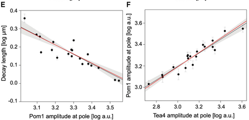
[[Image:Pom1 power laws.png| The power laws translate into lines in the log-log space. The power laws predicted by the model (red lines) closely match the experimental data (black dots and black regression lines) Left: For the relationship the gradient decay length and the Pom1 amplitude at the pole, the model predicts a -0.5 power law (red line) which is very closed to the observed power law of -0.52 (black line). Right: For the relationship between Pom1 and Tea4 amplitude at the pole, the model predicts a 2/3 power law (red line) which is very closed to the observed power law of 0.63 (black line). |thumb| left| 500px]] | [[Image:Pom1 power laws.png| The power laws translate into lines in the log-log space. The power laws predicted by the model (red lines) closely match the experimental data (black dots and black regression lines) Left: For the relationship the gradient decay length and the Pom1 amplitude at the pole, the model predicts a -0.5 power law (red line) which is very closed to the observed power law of -0.52 (black line). Right: For the relationship between Pom1 and Tea4 amplitude at the pole, the model predicts a 2/3 power law (red line) which is very closed to the observed power law of 0.63 (black line). |thumb| left| 500px]] | ||
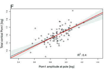
[[Image:Pom1_cortical.png| The power laws of 0.5 predicted by the model (red lines) between the total cortical Pom1 and the Pom1 amplitude at the pole closely match the experimental data of 0.46 (black dots and black regression lines). |thumb| 350px]] | [[Image:Pom1_cortical.png| The power laws of 0.5 predicted by the model (red lines) between the total cortical Pom1 and the Pom1 amplitude at the pole closely match the experimental data of 0.46 (black dots and black regression lines). |thumb| 350px]] | ||
| + | |||
| + | More details are available in the paper and the supplement. | ||
Revision as of 16:15, 14 July 2015
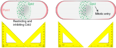
Fission yeast cells are rod-shaped cells that elongate until they reach a certain size (about 14 microns) and then split into two cells of equal size. This seems like a simple thing to do, but it begs the question of how does the cell know it has reached the right size and how can the cell know where its middle is. A few years ago, our collaborator Sophie Martin suggested a model that could explain those two processes, namely the timing (when to divide) and the positioning (where to divide) of cell division. According to that model (see Fig. on the right) the Pom1 kinase is constantly brought to the two poles of the cell and diffuses along the cortex of the cell. While it diffuses, it also detaches from the the cortex into the cytoplasm, such that the concentration of Pom1 at the cortex decreases towards the cell middle. In other words, it forms a gradient, or more precisely it forms a double gradient from each pole of the cell. Now, these gradients can be used as rulers, because the further away from the pole, the lower the concentration of Pom1. Indeed a molecular mechanism that is inhibited by Pom1 could only take place when Pom1 is is in sufficiently low concentration, that is when the cell is long enough, and also only in the cell middle, where Pom1 concentration is at its lowest. This molecular mechanism is implemented by the Cdr2 kinase that triggers mitotic entry unless which it inactivated by Pom1 phosphorylation.
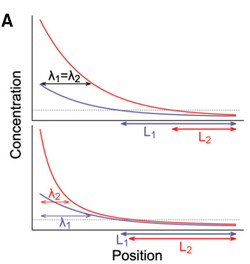
This is all nice (but still somewhat debated), but there is one issue. The amount of Pom1 that is brought to the cell tips is highly variable between cell and even within cells, such that the mechanism described above should be very imprecise. Indeed, if the Pom1 concentration at the pole varies a lot, this variation will be carried over to the cell middle, such that the Pom1 concentration will not be able to unambiguously indicate the distance to the pole. However, our collaborators had previously shown that Pom1 auto-phosphorylates multiple times, and that the affinity of Pom1 decreases with each phosphorylation. And this is where math comes in handy. Using a set of Partial Differential Equations (PDEs) we were able to show that if Pom1 auto-phosphorylation is intermolecular, i.e., a molecule of Pom1 can phosphorylate another molecule of Pom1 (not just itself), then the Pom1 gradient becomes a so-called power gradient. Power gradients have the special property that variations in concentration at one point of the gradient are attenuated and do not fully carry over downstream of the gradient (see Figure). Power gradients were hypothesized more than a decade ago as an abstract concept, but were not clearly observed in nature until now. Our paper shows theoretically that inter-molecular phosphorylation coupled to a phosphorylation dependent detachment (or decay) is a way to implement a power gradient.
But there is more to it. Since it is possible to find an analytical solution to our PDEs, we were able to extract three quantitative constitutive relations characteristic of our power gradient. Those constitutive relations are the following power laws:
- A power law of -0.5 between the length scale of the gradient and the amplitude of Pom1 at the pole.
- A power law of 2/3 between the amplitude of Pom1 and the amplitude of Tea4 at the pole
- A power law of 0.5 between the total cortical Pom1 and the amplitude of Pom1 at the pole
Those numbers do not depend on any particular parameters, there constitutive relations of our system. We then checked if we could observe those values experimentally by quantifying the concentration of Pom1 along the cortex of many cells. And, lo and behold, this is exactly what we observed: -0.52 for the first one, 0.63 for the second one and 0.46 for the third one (see Figures below). It is quite rare in biology that you can predict actual non-trivial numbers irrespectively of any parameters, and we do not think it is possible to find a different reasonable model that would account for those numbers. We thus believe that this work reveals the power of analytical computational models used with experimental data to validate biological hypotheses. Indeed there has been a growing concern among biologists that you can make many computational models say almost anything with suitable sets of parameters. Here we provide an example of computational model that makes quantitative and unambiguous predictions independently of the model parameters. The fact that those predictions precisely match our observations is a strongly supports the model. In our case, the model was further validated by showing in vivo and vitro that Pom1 auto-phosphorylates intermolecularly.

More details are available in the paper and the supplement.


