Predicting Blood Pressure from the retina using Deep Learning
File:Final Presentation Retina.pptx
Contents
Introduction
Background and Motivation
Heart disease has been the leading cause of death in the world for the last twenty years. It is therefore of great importance to look for ways to prevent it. In this project, funduscopy images of retinas of tens of thousands of participants collected by the UK biobank and data of biologically relevant variables collected in a dataset are used for two different purposes.
First, GWAS analysis of some of the variables in the dataset allows us to look at their concrete importance in the genome. Second, the dataset was used as a means of refining the selection of retinal images so that they could be subjected to a classification model called Dense Net with as output a prediction of hypertension. A key point associated with both of these analyses - especially for the classification part - is that mathematically adequate data cleaning should enhance the relevant GWAS p-values, or accuracy of hypertension prediction.
Data cleaning process
The data has been collected from the UK biobank and consists of :
1. Retina images of left eyes, right eyes, or both left and right eyes of the participants. Also, a few hundreds of participants have had replica images of either their left or right eye taken.
2. A 92366x47 dataset with rows corresponding to every left or right retina images. Columns refer to biologically relevant data previously measured on those images.
The cleaning process has involved :
1. Removing 15 variables by recommendation of the assistants and dividing the dataset into two : one (of size 78254x32) containing only participants which had both their left (labelled "L") and right (labelled "R") eyes taken and nothing else, and the other (of size 464x32) containing each replica (labelled "1") image alongside its original (labelled "0").
2. For every participants, every variables, and in the two datasets : applying <math> \delta = \frac{|L-R|}{L+R} </math> to the left-right dataset and <math> \delta = \frac{|0-1|}{0+1} </math> to the original-replica dataset. This delta computes the relative distance between either L and R, or 0 and 1.
3. Computing the T-test and the Cohen's D (the effect size) between each corresponding variables of the two datasets and removing the 5 variables with significant p-values after Bonferroni correction for 32 tests. This was done because for the classification model and to predict hypertension, it is better for input images of left and right eyes to not have striking differences between them, otherwise the machine could lose in accuracy by accounting for these supplementary data, instead of focusing on the overall structure of the images it analyses. We can check if each variable has a high left-right difference by comparing it to the corresponding variable 0-1 difference ; if a variable has a low left-right difference - a low delta (L, R) - its delta(L, R) distribution should be similarly distributed as its corresponding delta(0, 1) variable, because a replica has by definition no other difference with its original than the technical variability related to the way it was practically captured.
The classification has then used the 39127x27 delta(L, R) cleaned and transformed dataset for the selection of its images.
Deep Learning Model
This section focused on using the previously defined Delta variable to sort the images used as input for the classifier. A CNN model was built by the CBG to predict hypertension from retina fundus images. We wished to improve the predictions by reducing technical error in the input images. The statistical tests performed in the first part allow us to select the variable for which delta (L, R) can be used as an approximation of technical error (or delta (0, 1)), i.e select the variable with the smallest difference between delta (L, R) and delta (0, 1).
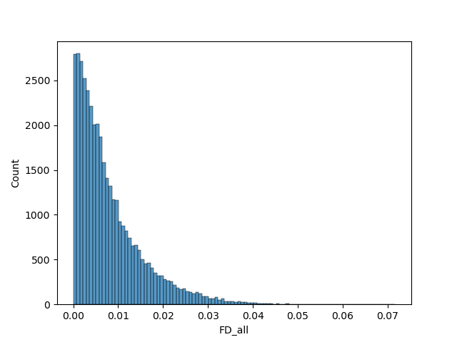
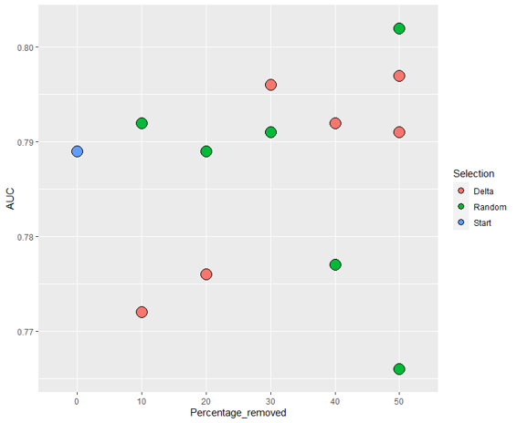
The delta values for the "FD_all" variable were used here to discriminate participants. Participants with the highest delta values were excluded. We ran the model with 10 different sets of images: Retaining 90%, 80%, 70%, 60% and 50% of images using the delta values, and random selection to make comparisons.
Results
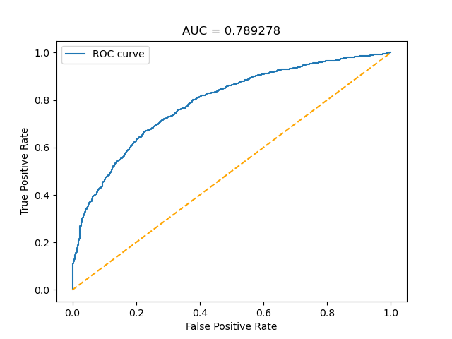
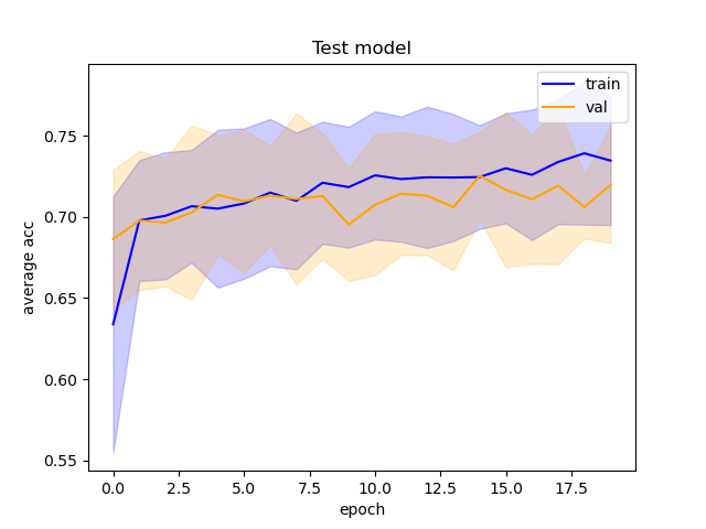
The ROC and training accuracy curves were extracted after every run. The shape of both curves didn't change much from run to run, but notable changes in AUROC were noted.
The AUC values for the different sets of images seem to follow a general trend: Decrease in precision as dataset size decreases for the randomly selected images, and increases when using delta.
However, the inherent variation in AUC results from run to run makes it hard to draw conclusions from such little data. Running the model at least thrice with each set of images would allow us to get a much clearer idea of what is actually happening, and to do statistical tests.
GWAS
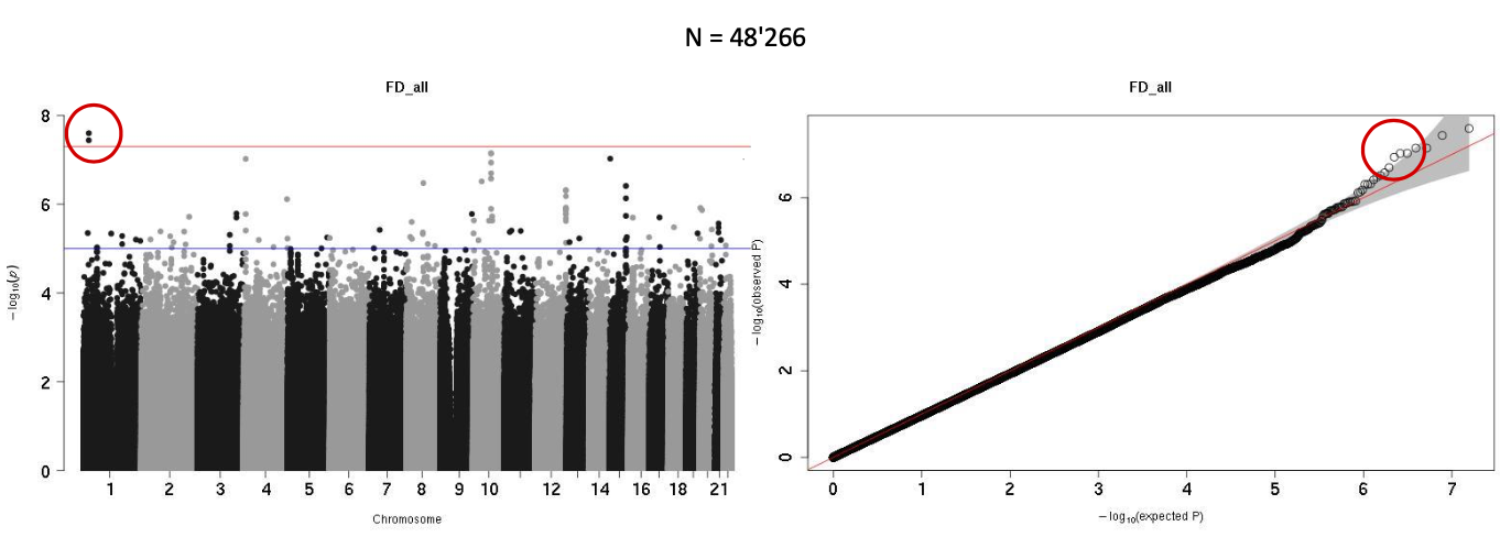
The goal of the GWAS was to investigate if the asymmetry of the eyes could have genetic origins. We decided to look at the variables with the largest left right difference were selected: Fractal dimension and tortuosity. The phenotype for the GWAS was the delta (delta = abs(L-R)/(L+R)) of fractal dimension and tortuosity. That way, we would we able to identify genes responsible for asymmetry in these variables. Two rounds of GWAS were made. The first one had approximately 40'000 subjects and the second one had approximately 50'000 subjects.
Results
The results were not significant. Only one GWAS was very slightly significant, the fractal dimension with the larger set of participants (indicated by red circle).
In the event of the GWAS showing a significant peak, we could have then investigated the part of the genome associated with it by looking up the reference SNP cluster ID (rSID) in NCBI. We could have then identified genes associated with fractal dimension asymmetry in the eyes.
