Difference between revisions of "Genetics of different body mass measurements"
(→Results of the genetic part) |
(→Conclusion) |
||
| (41 intermediate revisions by the same user not shown) | |||
| Line 10: | Line 10: | ||
<big>'''Phenotypic part'''</big> | <big>'''Phenotypic part'''</big> | ||
| + | |||
| + | '''Choice of phenotypes''' | ||
| + | |||
| + | The phenotypes we chose as definitions of obesity fall into 3 categories: BMI variants, waist based phenotypes and percentage of body fat. We defined them taking inspiration in the litterature[8,9]. The BMI variants category includes the canonical BMI (weight/height^2), as well as variants in which the power was changed to 1.6, 2.5 and 3. The rationale for 3 is the idea that the human body is a volume and not a surface, whereas 1.6 and 2.5 are values suggested by various authors to take into account the fact that taller people are not scaled up versions of small people. Waist circumference phenotypes are interesting as they take into account the location of the fat in the body, it is indeed known that visceral fat is more harmful than subcutaneous fat. This category includes waist circumference uncorrected, waist/hip ratio and waist/height ratio. Waist/hip ratio is a commonly measured characteristic, it is known to be different for men and women. The waist/height ratio is a try in correcting the waist circumference for the size of the person in a way that might be less sex sensitive. The percentage of body fat includes BAI [10] and RFM [11]. These two indexes are taken from two publications that measured % body fat by imaging techniques and derived equations to estimate it by simple measurement. | ||
| + | |||
| + | '''Linear regression''' | ||
| + | |||
| + | To see which of our phenotypes was the most correlated with systolic blood pressure, we performed several regressions with each of our phenotypes. We took into account the sex and age as counfounding factors. As the effect of the age is often non lienar, we also added the square of the age. | ||
| + | |||
| + | with interaction: SBP ~ phenotype * sex + age + age^2 | ||
| + | |||
| + | without interaction: SBP ~ phenotype + sex + age + age^2 | ||
| + | |||
| + | Background: SBP ~ sex + age + age^2 | ||
| + | |||
| + | We compared the model with and without interaction with sex. The phenotypes were normalized (F scores) so that the results of different phenotypes could be compared. We compared the phenotypes by looking at the adjusted R^2 and the regression coefficients. | ||
| + | The conditions for the validity of a linear regression are the homogeneity of the variance of the residues, the normality of the residues, the independence of the observations and the fact that the relationship is indeed linear. We checked these conditions using diagnostic plots (residual vs fitted, normal QQ plot, Scale location and residuals vs leverage). The conditions were respected for all the phenotypes. | ||
| Line 15: | Line 32: | ||
Still from the UK Biobank [4], we had data about individuals containing their characteristics, such as weight, height, ethnicity, …, and their SNPs (“Single Nucleotide Polymorphism”). We then performed a mini-GWAS on them | Still from the UK Biobank [4], we had data about individuals containing their characteristics, such as weight, height, ethnicity, …, and their SNPs (“Single Nucleotide Polymorphism”). We then performed a mini-GWAS on them | ||
| − | GWAS (Genome-Wide Association Study) is a statistical approach to identify the | + | |
| − | Indeed, GWAS contains all the SNPs and their p-value associated to the phenotype | + | GWAS (Genome-Wide Association Study) is a statistical approach to identify the significiance of a SNP for a certain trait/phenotype. |
| + | Indeed, GWAS contains all the SNPs and their p-value associated to the phenotype. | ||
| + | |||
As mentioned above, we worked on a mini-GWAS, meaning that it wasn’t about all the SNPs of the whole genome, it was a representative set of SNPs, which should normally give the same results as if we did it on the whole genome. | As mentioned above, we worked on a mini-GWAS, meaning that it wasn’t about all the SNPs of the whole genome, it was a representative set of SNPs, which should normally give the same results as if we did it on the whole genome. | ||
| + | |||
As the phenotypic part, we chose some covariants which we knew had an effect on the SNPs. By this way, we could see the phenotypic effect in a cruder way . | As the phenotypic part, we chose some covariants which we knew had an effect on the SNPs. By this way, we could see the phenotypic effect in a cruder way . | ||
We chose as covariants age, sex and genetic principal components (as ethnicity) | We chose as covariants age, sex and genetic principal components (as ethnicity) | ||
| Line 26: | Line 46: | ||
Then, we only kept the significant SNPs for each phenotype, and extracted the genes they belong to. By this way, we created some Venn diagrams to visualize how linked are the different genes between the different phenotypes | Then, we only kept the significant SNPs for each phenotype, and extracted the genes they belong to. By this way, we created some Venn diagrams to visualize how linked are the different genes between the different phenotypes | ||
| − | ==Results of the | + | ==Results of the phenotypic part== |
| Line 33: | Line 53: | ||
We started by exploring the distribution of our data. Based on the histograms, the variables seem to be either quite normally distributed (height) or a bit skewed to the right (weight, hip, waist). We also looked at the correlation between the variables visually thanks to scatterplots. Unsurprisingly, we see a clear correlation between BMI, waist circumference and hip circumference. The correlation is a lot less obvious with height, and seems completely absent between age and all other phenotypes. This is good, as it suggests that all age classes have a similar BMI, height, waist circumference and hip circumference distribution. | We started by exploring the distribution of our data. Based on the histograms, the variables seem to be either quite normally distributed (height) or a bit skewed to the right (weight, hip, waist). We also looked at the correlation between the variables visually thanks to scatterplots. Unsurprisingly, we see a clear correlation between BMI, waist circumference and hip circumference. The correlation is a lot less obvious with height, and seems completely absent between age and all other phenotypes. This is good, as it suggests that all age classes have a similar BMI, height, waist circumference and hip circumference distribution. | ||
| − | + | ||
'''Linear regression''' | '''Linear regression''' | ||
| − | + | The assumptions of the linear regression were not violated in all the phenotypes. We also checked that our phenotypes were not too correlated with the other variables; we can trust the model if the correlation is not higher than 0.7. The correlations are small enough for all the phenotypes out of RFM which already takes sex into account and has a correlation of nearly 1 with it. We therefore had to remove sex from the model. RFM is unarguably an interesting phenotype to study, but the way we designed our work does not really allow us to compare it with the others. | |
| − | |||
| − | |||
| − | |||
| − | |||
| − | |||
| − | |||
| − | We also checked that our phenotypes were not too correlated with the other variables; we can trust the model if the correlation is not higher than 0.7. The correlations are small enough for all the phenotypes out of RFM which already takes sex into account and has a correlation of nearly 1 with it. We | ||
| − | + | For all the phenotypes, we observed a significant and positive relationship with SBP, meaning that increasing of all our phenotypes is associated with a higher systolic blood pressure. The interaction of sex and phenotype was significant in all the cases. However, we observe that the general relationship is still similar in both sexes, as we generally have parallel curves, or only slightly different slopes. Moreover, we performed linear regressions both taking into account the interaction with the sex and without doing it and obtained overall similar results. For this reason, it may not be needed to stratify by sex. | |
| − | + | ''Figure 1 : Relationship between SBP and our phenotypes for men and women'' | |
| + | [[File:Figure_1.jpg]] | ||
For each model, we collected the effect of the phenotype as well as the adjusted R square of the model to which we subtracted the adjusted R square of the background model to estimate the variability explained by the phenotype. | For each model, we collected the effect of the phenotype as well as the adjusted R square of the model to which we subtracted the adjusted R square of the background model to estimate the variability explained by the phenotype. | ||
| − | Looking at this table, we obtain | + | Looking at this table, we obtain divergent results. On the one way, looking at the factors suggests that the waist based phenotypes explain best the systolic blood pressure (with respectively an increase of 3.44 points of SBP for each increase of 1 sd of waist circumference, 3.32 for waist/height and 3.24 for waist/hip ratio). BAI, BMI1.6 and BMI3 are associated with factors between 3.1 and 3.2, whereas BMI and BMI2.5 are associated with factors under 1. When looking at the adjusted R squares however, variants of the BMI explain a bigger part of the variability of SBP (2.82 % for BMI3, 2.77 % for BMI1.6 and BMI2.5, 2.65 % for BMI). As we have no arguments to decide which of the explained variance or the regression coefficient is the most clinically relevant, we cannot choose a best phenotype based on this only. |
| − | [ | + | ''Table 1 : Results of the linear regressions (model with interaction) for all phenotypes'' |
| + | [[File:Table_1.jpg]] | ||
| − | + | If we want to use the same phenotype for the whole population however, we can also look at the correlation of our phenotypes with sex and age. Indeed, if we don't want to stratify, we should select a phenotype that is not influenced to much by sex and age. in this case, BMI is way better than waist phenotypes, which have a correlation of around 15 % with age and even 65 % between sex and waist/hip ratio. | |
| − | |||
| − | |||
| − | |||
| − | |||
| − | |||
| − | |||
| − | |||
| − | |||
| + | ''Table 2 : Correlation of the phenotypes with sex and age'' | ||
| + | [[File:Table_2.jpg]] | ||
| + | One of the BMI variants might therefore be our most clinically relevant phenotype. these unclear results however illustrate well the difficulty of finding a good obesity measurment. Thi explains why BMI is still used by everyone even though its limits are known by everyone. | ||
==Results of the genetic part== | ==Results of the genetic part== | ||
| Line 73: | Line 83: | ||
A Manhattan plot displays the significant SNPs. SNPs are shown along the x-axis, sorted by chromosomes The relative negative logarithm of the association p-value for each SNP is displayed along the y-axis. Each SNP is thus represented with a dot. The strongest associations have the smallest p-value and thus their negative logarithm will be the greatest and high on the graph. All the SNP that are above the red line are significant. All the phenotypes show a lot of significant SNPs. All the phenotypes have similar results. We also see that there are more genes on the first chromosomes. | A Manhattan plot displays the significant SNPs. SNPs are shown along the x-axis, sorted by chromosomes The relative negative logarithm of the association p-value for each SNP is displayed along the y-axis. Each SNP is thus represented with a dot. The strongest associations have the smallest p-value and thus their negative logarithm will be the greatest and high on the graph. All the SNP that are above the red line are significant. All the phenotypes show a lot of significant SNPs. All the phenotypes have similar results. We also see that there are more genes on the first chromosomes. | ||
| − | 'Figure | + | ''Figure 2 : Four examples of Manhattan plot of our phenotypes'' |
[[File:manhattan.jpg]] | [[File:manhattan.jpg]] | ||
| Line 81: | Line 91: | ||
It is a different representation of the same results. A QQ plot plots the quantile distribution of observed p-values (on the y-axis) versus the quantile distribution of expected p-values. The SNPs here are all mixed, not sorted by chromosomes. All the SNP that are not on the red line are significant. The red line represents the probability of it occurring by chance. The plots are similar between the different phenotypes even if the upper right differs a little bit. Again, we see that a lot of SNPs are relevant with our phenotypes. | It is a different representation of the same results. A QQ plot plots the quantile distribution of observed p-values (on the y-axis) versus the quantile distribution of expected p-values. The SNPs here are all mixed, not sorted by chromosomes. All the SNP that are not on the red line are significant. The red line represents the probability of it occurring by chance. The plots are similar between the different phenotypes even if the upper right differs a little bit. Again, we see that a lot of SNPs are relevant with our phenotypes. | ||
| − | Figure | + | ''Figure 3 : Four examples of QQ plot of our phenotypes'' |
[[File:qq.jpg]] | [[File:qq.jpg]] | ||
| Line 90: | Line 100: | ||
As an example, it is known that the height is very heritable as its heritability is around 80% [6]. In our case, the waist-hip ratio has the lowest heritability as its at 13%. The BMI variations phenotypes have a heritability around 23%. The waist phenotypes have a heritability around 15%. Globally, all the phenotypes have a low heritability which make all the phenotypes interesting. | As an example, it is known that the height is very heritable as its heritability is around 80% [6]. In our case, the waist-hip ratio has the lowest heritability as its at 13%. The BMI variations phenotypes have a heritability around 23%. The waist phenotypes have a heritability around 15%. Globally, all the phenotypes have a low heritability which make all the phenotypes interesting. | ||
| − | Table 3 : | + | ''Table 3 : Heritability of our phenotypes'' |
[[File:her.jpg]] | [[File:her.jpg]] | ||
| Line 100: | Line 110: | ||
| − | At first | + | At first sighton the Fig.4, we can see that the majority of the genes are shared between the different phenotypes |
686 genes of them are shared between all phenotypes, which represents 11.3% | 686 genes of them are shared between all phenotypes, which represents 11.3% | ||
We also remark than BAI and weight have a lot of genes that are not shared with the other ones. | We also remark than BAI and weight have a lot of genes that are not shared with the other ones. | ||
| − | Figure | + | ''Figure 4: Venn diagram of the genes of the phenotypes'' |
[[File:Figure_6.jpg]] | [[File:Figure_6.jpg]] | ||
| − | We can see in a better way the repartition of the genes containing significatn SNPs in Fig. | + | We can see in a better way the repartition of the genes containing significatn SNPs in Fig.5 and Fig.6 |
| − | Figure | + | ''Figure 5: Venn diagram of the genes of the three categories'' |
[[File:Figure_7.jpg]] | [[File:Figure_7.jpg]] | ||
| − | Figure | + | ''Figure 6: Venn diagram of the genes of phenotypes in their own categories'' |
[[File:Figure_8.jpg]] | [[File:Figure_8.jpg]] | ||
| − | We found on “GWAS Catalog”[7] a list of different genes that have already been associated with systolic blood pressure (SBP). We made a Venn diagram (Fig. | + | We found on “GWAS Catalog”[7] a list of different genes that have already been associated with systolic blood pressure (SBP). We made a Venn diagram (Fig.7) to compare them with the genes containing significant SNPs we found above. |
On the 1962 SBP genes, 552 (28%) are shared with at least one of the phenotypes, and 125 (6.4%) are shared with all of them | On the 1962 SBP genes, 552 (28%) are shared with at least one of the phenotypes, and 125 (6.4%) are shared with all of them | ||
| − | Here is a table containing the number of shared gene between all the phenotypes and these SBP genes ( | + | Here is a table containing the number of shared gene between all the phenotypes and these SBP genes (Tab.4). We see that BAI is the phenotype which shares the highest number of genes with SBP genes, followed by BMI3 and BMI2.5 |
| − | Figure | + | ''Figure 7: Venn diagrams of the genes of our phenotypes and genes associated with SBP'' |
[[File:Figure_9.jpg]] | [[File:Figure_9.jpg]] | ||
| − | Table 4: Number of genes in common between the pehnotype and the SBP genes | + | ''Table 4: Number of genes in common between the pehnotype and the SBP genes'' |
[[File:Table_4.jpg]] | [[File:Table_4.jpg]] | ||
==Conclusion== | ==Conclusion== | ||
In conclusion, it is really difficult to find a good way to measure the obesity. A better phenotype than the usual BMI is not obvious, that is probably why the BMI is still commonly used even if it has some big bias. From our study, the different variants of the BMI phenotypes (BMI3, BMI1.6) are perhaps good phenotypes. They have a large R-squared and do not correlate a lot with the sex and the age. Also, a lot of SNP were found to be significant from the GWAS. Numerous genes were common to all the phenotype indicating that there is a genetic component of obesity. The heritability for all the phenotypes was around 20% which is not a lot. It means that the environment plays a big role and thus that we can have an influence on the phenotype. | In conclusion, it is really difficult to find a good way to measure the obesity. A better phenotype than the usual BMI is not obvious, that is probably why the BMI is still commonly used even if it has some big bias. From our study, the different variants of the BMI phenotypes (BMI3, BMI1.6) are perhaps good phenotypes. They have a large R-squared and do not correlate a lot with the sex and the age. Also, a lot of SNP were found to be significant from the GWAS. Numerous genes were common to all the phenotype indicating that there is a genetic component of obesity. The heritability for all the phenotypes was around 20% which is not a lot. It means that the environment plays a big role and thus that we can have an influence on the phenotype. | ||
| − | |||
Here is the link for our ppt presentation for additional information : | Here is the link for our ppt presentation for additional information : | ||
[[Media:ppt.pptx]] | [[Media:ppt.pptx]] | ||
| + | |||
| + | |||
| + | ''A special thank to Sofia Ortin Vela and Olga Trofimova for their supervising'' | ||
==References== | ==References== | ||
| Line 147: | Line 159: | ||
[6] https://www.nature.com/articles/d41586-019-01157-y#:~:text=For%20height%2C%20Visscher%20and%20colleagues,environmental%20factors%2C%20such%20as%20nutrition. | [6] https://www.nature.com/articles/d41586-019-01157-y#:~:text=For%20height%2C%20Visscher%20and%20colleagues,environmental%20factors%2C%20such%20as%20nutrition. | ||
| + | |||
| + | [7] : https://www.ebi.ac.uk/gwas/ | ||
| + | |||
| + | [8] : https://doi.org/10.1186/gm459 | ||
| + | |||
| + | [9] : https://journals.lww.com/00017285-201505000-00005 | ||
| + | |||
| + | |||
| + | [10] : http://doi.wiley.com/10.1038/oby.2011.38 | ||
| + | |||
| + | [11] : http://www.nature.com/articles/s41598-018-29362-1 | ||
Latest revision as of 10:58, 5 June 2022
File:Heritability of BMI Sofia.pdf
Contents
Introduction
Obesity is a "condition in which excess body fat has accumulated to such an extent that it may have a negative effect on health[1]". It is correlated to a lot of diseases, but particularly with cardiovascular diseases. They include heart attacks, strokes or even heart failures. The World Health Organization (WHO) states that cardiovascular diseases are the first cause of mortality in the world. 31% of deaths are attributable to cardiovascular diseases[2]. The systolic blood pressure is a potential indicator for these diseases. Finding a good definition of obesity seemed important. That is what we tried to do in the first part of the project. The most used definition is the BMI. This index is defined by dividing the weight by the square of the height. The BMI has a lot of limitations, so we tried to find another definition. We tried different combinations of diverse body measurements that potentially correlated to systolic blood pressure. The combinations are called the phenotypes. In the second part of the project, we performed a GWAS. That is an "observational study of a genome-wide set of genetic variants in different individuals to see if any variant is associated with a trait[3]". The study focused on associations between SNPs and our phenotypes which are potentially correlated to high systolic blood pressure. GWAS have already been performed on height, weight and BMI. The goal of this part was to see if other phenotypes showed better signals than BMI and bring different biology by looking at related genes. Heritability helped us also to determine whether a phenotype is relevant or not.
Methodology
Phenotypic part
Choice of phenotypes
The phenotypes we chose as definitions of obesity fall into 3 categories: BMI variants, waist based phenotypes and percentage of body fat. We defined them taking inspiration in the litterature[8,9]. The BMI variants category includes the canonical BMI (weight/height^2), as well as variants in which the power was changed to 1.6, 2.5 and 3. The rationale for 3 is the idea that the human body is a volume and not a surface, whereas 1.6 and 2.5 are values suggested by various authors to take into account the fact that taller people are not scaled up versions of small people. Waist circumference phenotypes are interesting as they take into account the location of the fat in the body, it is indeed known that visceral fat is more harmful than subcutaneous fat. This category includes waist circumference uncorrected, waist/hip ratio and waist/height ratio. Waist/hip ratio is a commonly measured characteristic, it is known to be different for men and women. The waist/height ratio is a try in correcting the waist circumference for the size of the person in a way that might be less sex sensitive. The percentage of body fat includes BAI [10] and RFM [11]. These two indexes are taken from two publications that measured % body fat by imaging techniques and derived equations to estimate it by simple measurement.
Linear regression
To see which of our phenotypes was the most correlated with systolic blood pressure, we performed several regressions with each of our phenotypes. We took into account the sex and age as counfounding factors. As the effect of the age is often non lienar, we also added the square of the age.
with interaction: SBP ~ phenotype * sex + age + age^2
without interaction: SBP ~ phenotype + sex + age + age^2
Background: SBP ~ sex + age + age^2
We compared the model with and without interaction with sex. The phenotypes were normalized (F scores) so that the results of different phenotypes could be compared. We compared the phenotypes by looking at the adjusted R^2 and the regression coefficients. The conditions for the validity of a linear regression are the homogeneity of the variance of the residues, the normality of the residues, the independence of the observations and the fact that the relationship is indeed linear. We checked these conditions using diagnostic plots (residual vs fitted, normal QQ plot, Scale location and residuals vs leverage). The conditions were respected for all the phenotypes.
Genotypic part
Still from the UK Biobank [4], we had data about individuals containing their characteristics, such as weight, height, ethnicity, …, and their SNPs (“Single Nucleotide Polymorphism”). We then performed a mini-GWAS on them
GWAS (Genome-Wide Association Study) is a statistical approach to identify the significiance of a SNP for a certain trait/phenotype. Indeed, GWAS contains all the SNPs and their p-value associated to the phenotype.
As mentioned above, we worked on a mini-GWAS, meaning that it wasn’t about all the SNPs of the whole genome, it was a representative set of SNPs, which should normally give the same results as if we did it on the whole genome.
As the phenotypic part, we chose some covariants which we knew had an effect on the SNPs. By this way, we could see the phenotypic effect in a cruder way . We chose as covariants age, sex and genetic principal components (as ethnicity)
Then, we used these different GWAS to represent the relevant SNPs on a Manhattan plot and QQ plot. We also compute the heritability of the different phenotypes, to have an idea on the impact we could have on our environment to improve the health.
Then, we only kept the significant SNPs for each phenotype, and extracted the genes they belong to. By this way, we created some Venn diagrams to visualize how linked are the different genes between the different phenotypes
Results of the phenotypic part
Data exploration
We started by exploring the distribution of our data. Based on the histograms, the variables seem to be either quite normally distributed (height) or a bit skewed to the right (weight, hip, waist). We also looked at the correlation between the variables visually thanks to scatterplots. Unsurprisingly, we see a clear correlation between BMI, waist circumference and hip circumference. The correlation is a lot less obvious with height, and seems completely absent between age and all other phenotypes. This is good, as it suggests that all age classes have a similar BMI, height, waist circumference and hip circumference distribution.
Linear regression
The assumptions of the linear regression were not violated in all the phenotypes. We also checked that our phenotypes were not too correlated with the other variables; we can trust the model if the correlation is not higher than 0.7. The correlations are small enough for all the phenotypes out of RFM which already takes sex into account and has a correlation of nearly 1 with it. We therefore had to remove sex from the model. RFM is unarguably an interesting phenotype to study, but the way we designed our work does not really allow us to compare it with the others.
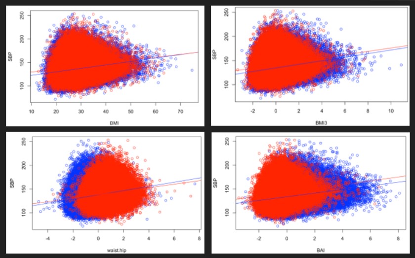
For all the phenotypes, we observed a significant and positive relationship with SBP, meaning that increasing of all our phenotypes is associated with a higher systolic blood pressure. The interaction of sex and phenotype was significant in all the cases. However, we observe that the general relationship is still similar in both sexes, as we generally have parallel curves, or only slightly different slopes. Moreover, we performed linear regressions both taking into account the interaction with the sex and without doing it and obtained overall similar results. For this reason, it may not be needed to stratify by sex.
Figure 1 : Relationship between SBP and our phenotypes for men and women
For each model, we collected the effect of the phenotype as well as the adjusted R square of the model to which we subtracted the adjusted R square of the background model to estimate the variability explained by the phenotype. Looking at this table, we obtain divergent results. On the one way, looking at the factors suggests that the waist based phenotypes explain best the systolic blood pressure (with respectively an increase of 3.44 points of SBP for each increase of 1 sd of waist circumference, 3.32 for waist/height and 3.24 for waist/hip ratio). BAI, BMI1.6 and BMI3 are associated with factors between 3.1 and 3.2, whereas BMI and BMI2.5 are associated with factors under 1. When looking at the adjusted R squares however, variants of the BMI explain a bigger part of the variability of SBP (2.82 % for BMI3, 2.77 % for BMI1.6 and BMI2.5, 2.65 % for BMI). As we have no arguments to decide which of the explained variance or the regression coefficient is the most clinically relevant, we cannot choose a best phenotype based on this only.
Table 1 : Results of the linear regressions (model with interaction) for all phenotypes

If we want to use the same phenotype for the whole population however, we can also look at the correlation of our phenotypes with sex and age. Indeed, if we don't want to stratify, we should select a phenotype that is not influenced to much by sex and age. in this case, BMI is way better than waist phenotypes, which have a correlation of around 15 % with age and even 65 % between sex and waist/hip ratio.
Table 2 : Correlation of the phenotypes with sex and age

One of the BMI variants might therefore be our most clinically relevant phenotype. these unclear results however illustrate well the difficulty of finding a good obesity measurment. Thi explains why BMI is still used by everyone even though its limits are known by everyone.
Results of the genetic part
Manhattan plots
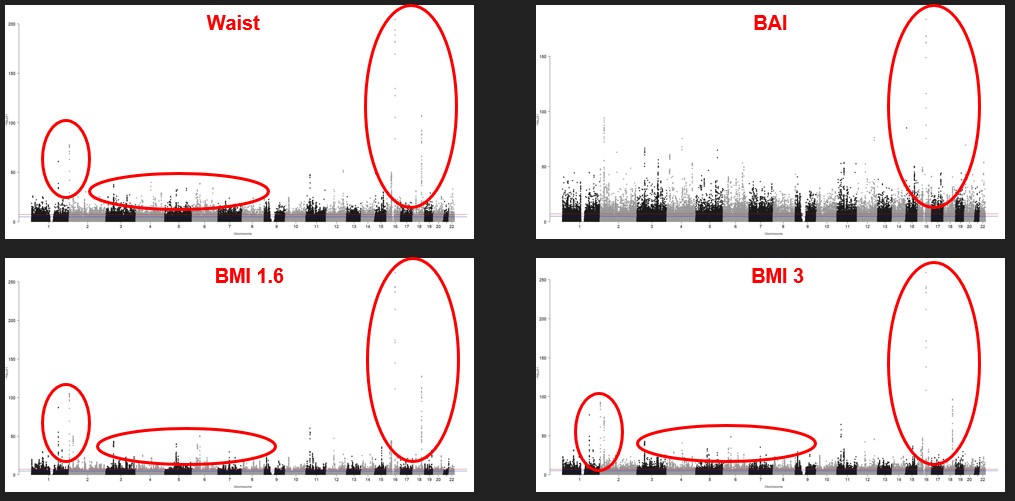
A Manhattan plot displays the significant SNPs. SNPs are shown along the x-axis, sorted by chromosomes The relative negative logarithm of the association p-value for each SNP is displayed along the y-axis. Each SNP is thus represented with a dot. The strongest associations have the smallest p-value and thus their negative logarithm will be the greatest and high on the graph. All the SNP that are above the red line are significant. All the phenotypes show a lot of significant SNPs. All the phenotypes have similar results. We also see that there are more genes on the first chromosomes.
Figure 2 : Four examples of Manhattan plot of our phenotypes
Qq plots
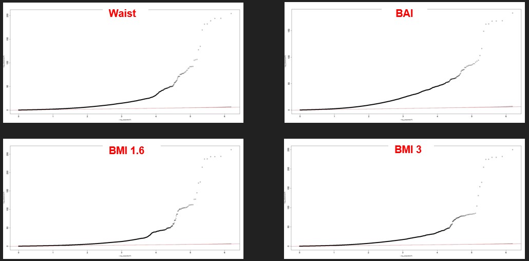
It is a different representation of the same results. A QQ plot plots the quantile distribution of observed p-values (on the y-axis) versus the quantile distribution of expected p-values. The SNPs here are all mixed, not sorted by chromosomes. All the SNP that are not on the red line are significant. The red line represents the probability of it occurring by chance. The plots are similar between the different phenotypes even if the upper right differs a little bit. Again, we see that a lot of SNPs are relevant with our phenotypes.
Figure 3 : Four examples of QQ plot of our phenotypes
Heritability
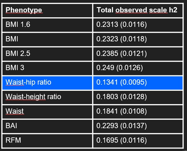
From the GWAS we performed we also calculated the heritability of each phenotype. The heritability can be defined such as the « amount of phenotypic (observable) variation in a population that is attributable to individual genetic differences » [5]. A phenotype is explained by phenotypic variation, genetic variation and random effects. If the heritability is very high, it means that the phenotype is a lot attributable to individual genetic differences and thus that the environment has a low impact. For us, as we want to have influence on the phenotype, the phenotypes with a low heritability are more interesting. As an example, it is known that the height is very heritable as its heritability is around 80% [6]. In our case, the waist-hip ratio has the lowest heritability as its at 13%. The BMI variations phenotypes have a heritability around 23%. The waist phenotypes have a heritability around 15%. Globally, all the phenotypes have a low heritability which make all the phenotypes interesting.
Table 3 : Heritability of our phenotypes
Venn Diagrams
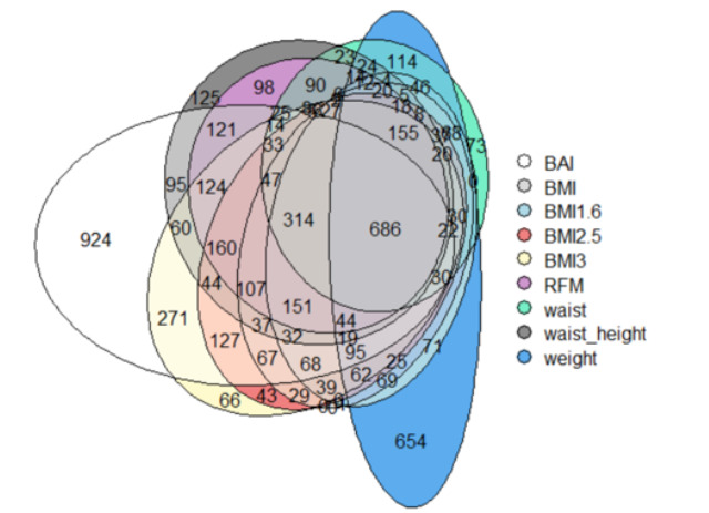
When confronting all the genes of all phenotypes, a total of 6097, we wanted to visualize how they were dispersed between all the phenotypes.
At first sighton the Fig.4, we can see that the majority of the genes are shared between the different phenotypes
686 genes of them are shared between all phenotypes, which represents 11.3%
We also remark than BAI and weight have a lot of genes that are not shared with the other ones.
Figure 4: Venn diagram of the genes of the phenotypes
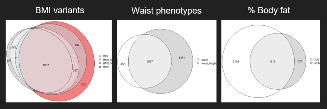
We can see in a better way the repartition of the genes containing significatn SNPs in Fig.5 and Fig.6
Figure 5: Venn diagram of the genes of the three categories
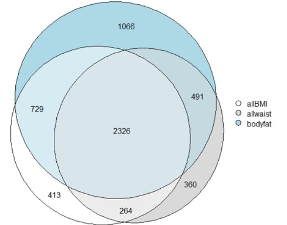
Figure 6: Venn diagram of the genes of phenotypes in their own categories
We found on “GWAS Catalog”[7] a list of different genes that have already been associated with systolic blood pressure (SBP). We made a Venn diagram (Fig.7) to compare them with the genes containing significant SNPs we found above.
On the 1962 SBP genes, 552 (28%) are shared with at least one of the phenotypes, and 125 (6.4%) are shared with all of them
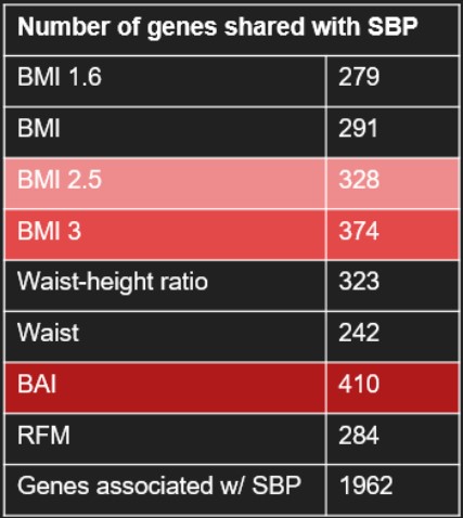
Here is a table containing the number of shared gene between all the phenotypes and these SBP genes (Tab.4). We see that BAI is the phenotype which shares the highest number of genes with SBP genes, followed by BMI3 and BMI2.5
Figure 7: Venn diagrams of the genes of our phenotypes and genes associated with SBP
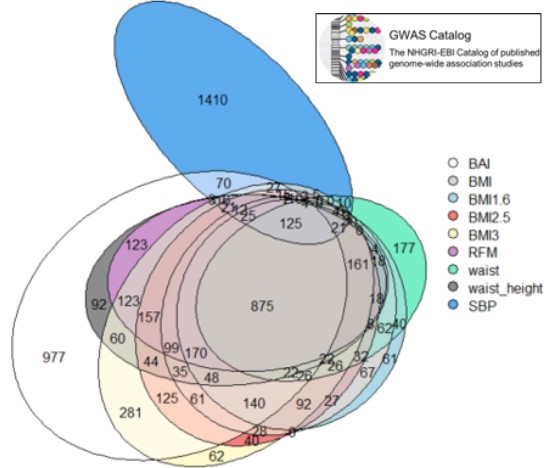
Table 4: Number of genes in common between the pehnotype and the SBP genes
Conclusion
In conclusion, it is really difficult to find a good way to measure the obesity. A better phenotype than the usual BMI is not obvious, that is probably why the BMI is still commonly used even if it has some big bias. From our study, the different variants of the BMI phenotypes (BMI3, BMI1.6) are perhaps good phenotypes. They have a large R-squared and do not correlate a lot with the sex and the age. Also, a lot of SNP were found to be significant from the GWAS. Numerous genes were common to all the phenotype indicating that there is a genetic component of obesity. The heritability for all the phenotypes was around 20% which is not a lot. It means that the environment plays a big role and thus that we can have an influence on the phenotype.
Here is the link for our ppt presentation for additional information : Media:ppt.pptx
A special thank to Sofia Ortin Vela and Olga Trofimova for their supervising
References
[1] https://en.wikipedia.org/wiki/Obesity
[3] https://en.wikipedia.org/wiki/Genome-wide_association_study
[4] https://www.ukbiobank.ac.uk/
[5] https://www.britannica.com/science/heritability
[7] : https://www.ebi.ac.uk/gwas/
[8] : https://doi.org/10.1186/gm459
[9] : https://journals.lww.com/00017285-201505000-00005