Which unwanted factors influence laboratory mice?

Informations

By: Leticia Wüthrich and Martin Quintas.

Supervisor: Frédéric Schütz.

Link to presentation: https://docs.google.com/presentation/d/1EEJKlP73pZFCd6OF_fqTT9LVO_TrEVl3JDRN23b1BYE/edit?usp=sharing

Introduction

Mice play a crucial role in a wide range of research contexts, from genetic studies to drug development. While it is often assumed that genetically identical mice are clones of one another, this is not always true. Environmental differences, such as cage effects, can influence the mice. These cage effects can stem from various factors, including different environmental conditions between cages, social interactions, varying microbial exposures, and even how the cages are handled or maintained. Cage effects contribute to variation among mice, often resulting in greater similarity among mice within the same cage and greater differences between mice from different cages.

Initial Simulations

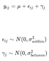
To illustrate the impact of cage effects on experimental data analysis, we perform simulations for the weights of mice in two different groups, distributed in a hierarchical design, based on the following formula:

Thus, ϵij represents the inter-individual variance for the i-th mouse within the j-th cage, and γj represents the variance specific to the j-th cage that affects all mice within that cage.

Essentially, each data point is created based on a certain mean 𝑢, to which we add random inter-individual variance. Additionally, based on the cage where the mice are housed, another random source of variance is added, which is the same for all mice within the same cage. This is modeled using a normal distribution. The treatment effect represents the mean difference between the two groups of mice, so it impacts the 𝑢 parameter.

Simulations conducted with and without a cage effect and with and without a treatment effect reveal that the presence of both a treatment effect and a cage effect increases the likelihood of false negatives. Conversely, the presence of a cage effect without a treatment effect increases the likelihood of false positives.

1. (See slides 15-18 of the presentation)

Note: in these simulations, when there was a treatment or cage effect, these were set to 5 grams.

Goals of the Project

The main goals of the project were to determine if there was an effect of the cages on the weight of the mice in a dataset that we received. If there was a cage effect, we wanted to quantify it, extract the variance explained by this effect and perform some more simulations to really understand how to deal with it. Finally, the goal was to improve the experimental design in order to make the cage effect as little as possible.

Data Description

Our dataset came for real-life data from mice of the Frédéric Preitner research group. In the dataset we had 88 rows representing 88 mice distributing into 19 cages. We had the genotype for two genes (GLP1Rc and GIPRc) and the weight of each individual. For the GLP1Rc gene, there was 2 possible genotypes and for the GIPRc there was 3 possible genotypes but all combinations of genotypes were not proposed in our mice. Note that individuals of the same cage always had the same genotype but individuals of the same genotype could be distributed into several cages. This describes a hierarchical design were the cage is nested into the genotype. Since we are not interested in the genotype effect on the weight of the mice, we decided to combine both genotypes.

Data visualization

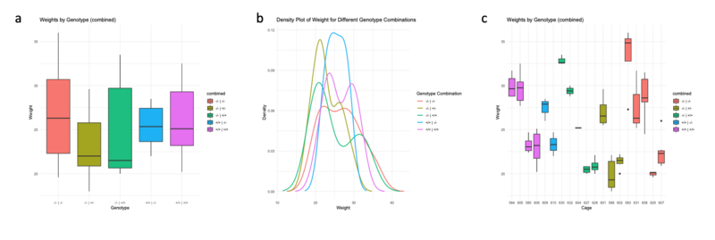
First, let's visualize the distribution of the weight of the mice with a boxplot (figure 1a). Here we see that there is a quite large variance inside the genotypes but globally there are no big differences between the groups. When we visualize the data with a density plot (figure 1b), we distinguish several bumps within the genotypes. These bumps indicate a potential effect of the cages inside the genotypes. Finally, by visualizing the data by cage (figure 1c), we see that inside genotypes, there is a big variance but we also see that this variance is much smaller inside the cages.

Figure 1: distribution of the weight of the mice according to the combined genotype. a, boxplot of the distribution by genotype. b, density plot of the distribution by genotype. c, boxplot of the distribution by cage (boxes of the same color represent cages where we find mice of the same genotype).

Results

Statistical Analysis

To quantify this cage effect, we performed the two ANOVAs and compared the variance of the residuals and the p-value of the genotype effect.

Table 1: variance of the residuals and p-values of the genotype effect of both ANOVAs performed on the data

Test	Variance (residuals)	p-value (genotype)
One-way ANOVA	18.7	0.05
Hierarchical ANOVA	3.3	2e-8

When the cages are taken into account we see that both the variance of the residuals and the p-value of the genotype effect decrease a lot. We see that just by taking cages into account, the variance of the residuals is much smaller and that the effect of the genotype is now much more significant. This means that there is a significant effect of the cages on the weight of the mice. From the hierarchical ANOVA, we extracted the standard deviation due to the cage effect which was estimated at 8.5g. This value will be useful to perform some more simulations.

Final Simulations

To determine how to account for the cage effect, we considered three different types of statistical models:

1. When the cage effect is not considered
2. Fixed effects models
3. Mixed effects models

We used the same simulations as before but adapted them to our statistical models. Initially, we applied parameters that reflect our data, setting the cage effect to 8.5g (calculated from ANOVA), with 4 cages and 4 mice per cage. The false positive rates and power we obtained were as follows:

1. (See slide 64 of the presentation)

None of the statistical models performed particularly well, likely due to the large cage effect.

This led us to question how the experimental design could be improved to reduce the impact of the cage effect on model performance. We conducted numerous simulations (around 50 or 60) to explore this. Generally, we found that power and false positive rates improve if:

1. The cage effect is smaller
2. The treatment effect is larger
3. The number of cages is increased
4. The number of mice per cage is decreased

The only parameters we can realistically control in the experimental design are the number of cages and the number of mice per cage.

When we increased the number of cages and decreased the number of mice per cage, the performance of the models improved:

1. (See slide 74 of the presentation)

For comparison, with the same total number of mice and the same cage effect, but with fewer cages and more mice per cage, the performance of the models was much worse:

1. (See slide 75 of the presentation)

Thus, with improved experimental design, only the mixed models became truly appropriate for data with a cage effect as large as ours.

Conclusion

We hope we were able to convince you that cage effects are very real and have a significant impact on the interpretation of data. These effects must be accounted for with an appropriate statistical model, which can depend on various factors, though mixed models are generally the best choice. However, improving the experimental design—particularly by reducing the number of mice per cage and increasing the number of cages per treatment—can greatly reduce the impact of cage effects on the performance of statistical models.