Retinal vasculature
Project presented by Leïla Ouhamma & Audran Feuvrier
Supervised by Daniel Krefl
Introduction
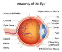
The Retinal vasculature (RV) refers to the blood vessels that supply the retina, which is the thin layer of tissue located at the back of the eye.
It is responsible for detecting light and sending visual information to the brain.
The retinal vasculature includes both arteries and veins, which branch out from the optic nerve and supply oxygen and nutrients to the retina.
The advantage in working with RV
There is a significant interest in working with RV. These blood vessels can provide important diagnostic information about the health of the eye and the body as a whole. Changes in the RV can be a sign of various medical conditions, including diabetes, hypertension, and cardiovascular disease. Therefore, the examination of the retinal vasculature is an important part of a comprehensive eye exam and can help detect and monitor these conditions.
Moreover, obtaining images of the retinal vasculature can be relatively easy and cost-effective with modern technology, such as during a routine exam at the ophtalmologist. There are various methods known to be non-invasive and generally well-tolerated by patients.
Deep Learning: Revealing Insights through RV image embedding
Our aim is to use deep learning auto-encoder on the retinal vasculature images to produce an RV embedding space, enabling us to gain insights on our RV images.
To do so, we will first build DL algorithms to produce a latent space to detect and highlight specific features.
Then, the results can be used to learn about the behavior of the algorithm, use this latent space for potential inference on diagnostics and genetic correlation.
Milestones of the project
1. Data pre-processing
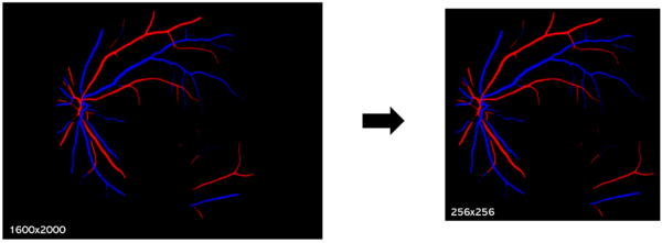
In the case of RV images, images have been previously segmented to identify veins and arteries. A few processing steps were left to do before they were usable for the auto-encoder machine.
- Cropping: A first step is to crop the image. This involves defining a cropping area to get rid of non relevant information.
- Resizing: The next step is to resize the image to a standard size. This is done to ensure that all images have the same dimensions and to reduce the computational load during subsequent analysis.
- Color changes: Finally we did a grey scaling standardization. We also prepared pictures containing only the veins and arteries to train our model on each structure because maybe it could show unexpected features which could affect the accuracy of subsequent analysis.
2. Build and train the model
When the data is ready, we define the auto-encoder we want to use. An auto-encoder is a type of artificial neural network architecture that learns a compressed representation of data by mapping it to a lower-dimensional latent space and then reconstructing the original data from this lower-dimensional representation. In the context of RV images, an auto-encoder can be used for unsupervised feature learning.
The encoder takes the input image and maps it to a lower-dimensional latent space, while the decoder takes the latent space representation and reconstructs the original image.
We also base our machine training on a Convolutional Neural Network (CNN) model. It uses a convolutional encoder with convolution layers to extract image features and pooling layers to reduce image size. Then, it uses a convolutional decoder with deconvolution/upsampling layers to reconstruct and enhance details.
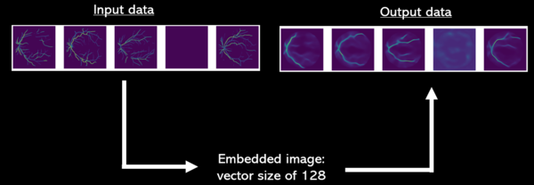
The auto-encoder is based on a U-net architecture for segmentation, which combines the two previous concepts to divide each image into several distinct regions, so that they can be analyzed separately. The embedding of RV images consists in representing the visual features of images in the form of compact, low-dimensional vectors (size of the vectors: 128). This allows the capture of essential image information in an easy-to-understand, compact form, facilitating subsequent analysis. We will use these values for the analysis section.
Thanks to Fig.3 one may have a better understand of how the machine works and embedding it produces. Pictures of predicted images have been taken at epoch 17.
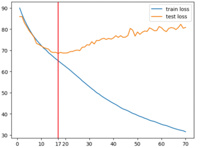
Our machine has been trained on 10 000 RV images from both left and right eyes equally. The cost function of our model is the Mean Squared Error between our input RV images and the predicted RV images of the model (cf. Fig.3 for comparison of input images and predicted images). To find the optimal number of training epochs of our model we have plotted the training MSE loss against the test MSE loss.
Thanks to Fig.4 we see that after epoch number 17 the model starts overfitting. So epoch number 17 is the optimal training epoch for the model to be used for subsequent embedding analysis.
Results
3. Analysis using the embeddings
Now that the machine is trained we have produced the embedding space by feeding through 30 000 test RV images from which we have obtained 30 000 embedding vectors of size 128. This makes our embedding space 128 dimensions so we must use dimensionality reduction algorithms to visualize structure in the data. t-SNE is an appropriate model to use for dimensionality reduction because as it is non-linear it is able to preserve local and global structures within the data.
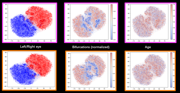
One can see on Fig. 5 that two clusters have been formed well separating left and right eyes. Within these 2 clusters, when colored by the normalized number of vessel bifurcation in the RV image, a gradient can be seen with the higher level of vessel bifurcations being put the extremities of the clusters and the lower number of bifurcations are put closer together towards the middle. Moreover a keen eye may notice a correlation between the number of vessel bifurcations and the age associated with the sample because the older the sample the less the number of bifurcations. Finally controlling for age and sex seems to have not had a strong effect on the t-SNE representation. As we have substracted age and sex effect by a multiple regression onto 128 variables simultaneously one may want to try to substract age and sex effect using a linear regression model and controlling the effect one variable after the other instead.
Fig.5 seems to hint that the embedding seems to preserve information of the images' phenotypes like the number of bifurcations.
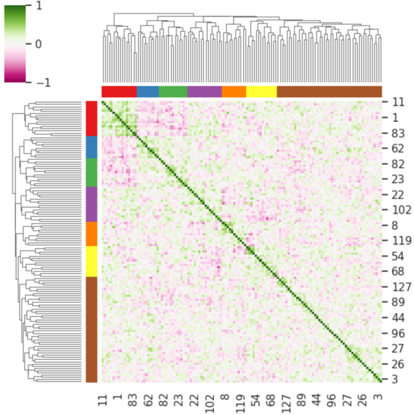
Fig.6 is a clustermap of the correlation matrix between each embedding variables. One can see clusters of well correlated variables suggesting the presence of structure in the data. These clusters could explain some features of the images like classical phenotypes such as tortuosity, vessel diameter, bifurcations and left or right eye. A deeper look into the images' phenotypes may give us some insight as to how and what information the machine learns and preserves to reconstruct a predicted image.
Conclusion
Preliminary analysis of the machine's results seems to indicate promising usability of the embedding space for potential inference on correlation with some image's phenotypes such as number of bifurcations and others. If it were proved to be meaningful by a more thorough analysis it would give important insight as to what the model learns and how it behaves. Other analysis like the training of a classifier on the embedding space for potential predictability of vascular diseases could show promising results. The possibility of using the embedding for potential genetic correlations would be interesting for gaining insights into one's genotype simply by a retinal vasculature image.
