Difference between revisions of "Retinal vasculature"
(→Milestones of the project) |
(→Milestones of the project) |
||
| Line 42: | Line 42: | ||
<small>Thanks to Fig.3 one may have a better understand of how the machine works and embedding it produces. Pictures of predicted images have been taken at epoch 17. | <small>Thanks to Fig.3 one may have a better understand of how the machine works and embedding it produces. Pictures of predicted images have been taken at epoch 17. | ||
| − | <small>Our machine has been trained on 10 000 RV images from both left and right eyes equally. The cost function of our model is the Mean Squared Error between our input RV images and the predicted RV images of the model (cf. Fig.3 for comparison of input images and predicted images). To find the optimal number of training epochs of our model we have plotted the training MSE loss against the test MSE loss. | + | <small>Our machine has been trained on 10 000 RV images from both left and right eyes equally. The cost function of our model is the Mean Squared Error between our input RV images and the predicted RV images of the model (cf. Fig.3 for comparison of input images and predicted images). To find the optimal number of training epochs of our model we have plotted the training MSE loss against the test MSE loss. |
[[File:MSE.png|thumb|center|400px|<small>'''Fig.4:''' Average Mean Squared Error per epoch</small>]] | [[File:MSE.png|thumb|center|400px|<small>'''Fig.4:''' Average Mean Squared Error per epoch</small>]] | ||
| − | <small>Thanks to Fig.4 we see that after epoch number 17 the model starts overfitting. So epoch number 17 is the optimal training epoch for the model to be used for subsequent embedding analysis. | + | <small>Thanks to Fig.4 we see that after epoch number 17 the model starts overfitting. So epoch number 17 is the optimal training epoch for the model to be used for subsequent embedding analysis. |
== '''Results''' == | == '''Results''' == | ||
Revision as of 11:46, 28 May 2023
Project presented by Leïla Ouhamma & Audran Feuvrier
Supervised by Daniel Krefl
Introduction
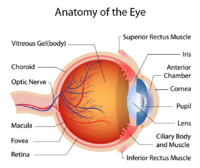
The Retinal vasculature (RV) refers to the blood vessels that supply the retina, which is the thin layer of tissue located at the back of the eye.
It is responsible for detecting light and sending visual information to the brain.
The retinal vasculature includes both arteries and veins, which branch out from the optic nerve and supply oxygen and nutrients to the retina.
The advantage in working with RV
There is a significant interest in working with RV. These blood vessels can provide important diagnostic information about the health of the eye and the body as a whole. Changes in the RV can be a sign of various medical conditions, including diabetes, hypertension, and cardiovascular disease. Therefore, the examination of the retinal vasculature is an important part of a comprehensive eye exam and can help detect and monitor these conditions.
Moreover, obtaining images of the retinal vasculature can be relatively easy and cost-effective with modern technology, such as during a routine exam at the ophtalmologist. There are various methods known to be non-invasive and generally well-tolerated by patients.
Deep Learning: Revealing Insights through RV image embedding
Our aim is to use deep learning auto-encoder on the retinal vasculature images to produce an RV embedding space, enabling us to gain insights on our RV images.
To do so, we will first build DL algorithms to produce a latent space to detect and highlight specific features.
Then, the results can be used to learn about the behavior of the algorithm, use this latent space for potential inference on diagnostics and genetic correlation.
Milestones of the project
1. Data pre-processing
In the case of RV images, images have been previously segmented to identify veins and arteries. A few processing steps were left to do before they were usable for the auto-encoder machine.
- Cropping: A first step is to crop the image. This involves defining a cropping area to get rid of non relevant information.
- Resizing: The next step is to resize the image to a standard size. This is done to ensure that all images have the same dimensions and to reduce the computational load during subsequent analysis.
- Color changes: Finally we did a grey scaling standardization. We also prepared pictures containing only the veins and arteries to train our model on each structure because maybe it could show unexpected features which could affect the accuracy of subsequent analysis.
2. Build and train the model
When the data is ready, we define the auto-encoder we want to use. An auto-encoder is a type of artificial neural network architecture that learns a compressed representation of data by mapping it to a lower-dimensional latent space and then reconstructing the original data from this lower-dimensional representation. In the context of RV images, an auto-encoder can be used for unsupervised feature learning.
The encoder takes the input image and maps it to a lower-dimensional latent space, while the decoder takes the latent space representation and reconstructs the original image.
We also base our machine training on a Convolutional Neural Network (CNN) model. It uses a convolutional encoder with convolution layers to extract image features and pooling layers to reduce image size. Then, it uses a convolutional decoder with deconvolution/upsampling layers to reconstruct and enhance details.
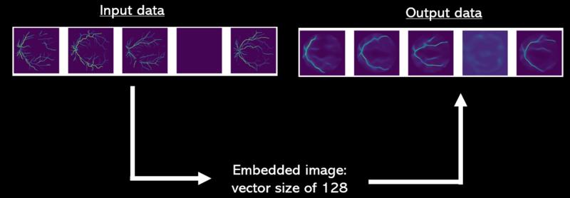
The auto-encoder is based on a U-net architecture for segmentation, which combines the two previous concepts to divide each image into several distinct regions, so that they can be analyzed separately. The embedding of RV images consists in representing the visual features of images in the form of compact, low-dimensional vectors (size of the vectors: 128). This allows the capture of essential image information in an easy-to-understand, compact form, facilitating subsequent analysis. We will use these values for the analysis section.
Thanks to Fig.3 one may have a better understand of how the machine works and embedding it produces. Pictures of predicted images have been taken at epoch 17.
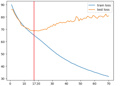
Our machine has been trained on 10 000 RV images from both left and right eyes equally. The cost function of our model is the Mean Squared Error between our input RV images and the predicted RV images of the model (cf. Fig.3 for comparison of input images and predicted images). To find the optimal number of training epochs of our model we have plotted the training MSE loss against the test MSE loss.
Thanks to Fig.4 we see that after epoch number 17 the model starts overfitting. So epoch number 17 is the optimal training epoch for the model to be used for subsequent embedding analysis.
Results
3. Analysis using the embeddings
Conclusion


